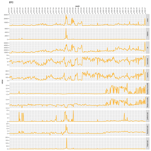
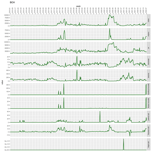
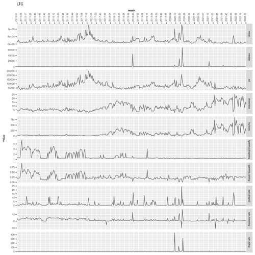
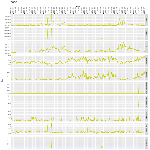
I’ve performed some statistical analysis of spent output age for BTC, BCH, LTC, and DOGE since 2015 to inform an improved Monero decoy selection algorithm. I don’t think anything actionable for BCH directly comes from this research, but it’s interesting nevertheless. This analysis is related to the “coin days destroyed” metric, although I take into account only the age of outputs and not their value.
To me, the main surprises in the analysis are:
-
The age distribution for all examined blockchains is quite unstable from week to week. In general I expected a sort of gradual evolutionary trend over time. The variability probably is caused by exchange rate volatility. The instability of the distributions is more consistent with use of these coins as speculative assets rather than as everyday peer-to-peer electronic cash.
-
There was not a strong correlation between blockchains in the movement over time of the mean nor standard deviation of the age distributions. However, there was a substantial correlation for the skewness and kurtosis, which correspond to the 3rd and 4th statistical moments of distributions. This makes some sense since skewness and kurtosis describe what is happening in the tails of distributions. When there is cryptosphere-wide volatility in the cryptocurrency exchange rates, it is likely for old coins of all blockchains to “wake up” and participate in speculative activity in exchanges. I expected to see the correlations in the means, too, however.
Due to formatting and gif files size issues, I omit the “Evaluation of forecast accuracy” and “Animated evolution of distributions” sections on this forum post. Those sections are in the full write-up here:
https://rucknium.me/html/spent-output-age-btc-bch-ltc-doge.html
Some of the summary statistics are available in CSV format here. The R code to produce the analysis is here, but note that several terabytes of storage and perhaps 256GB of RAM would be needed to reproduce the analysis.
Summary characterization of distributions over time
The first set of graphs show several statistics about the age of spent outputs of BTC, BCH, LTC, and DOGE since 2015. The age units are in terms of blocks. For BTC and BCH the interval between blocks is 10 minutes. For LTC it is 2.5 minutes and for DOGE it is 1 minute. The unit of observation is the ISO week, a natural unit of economic time.
The first line graphs show the mean, median, standard deviation, skewness, and kurtosis. The skewness and kurtosis statistics may be unfamiliar. They are the third and fourth standardized moments of a distribution, respectively. The moments of a distribution is defined by a power of the expectation \mathrm{E}[X] , i.e. theoretical mean, of the distribution. The k th moment is \mathrm{E}[X^{k}] . Moments extend the concept of moving from expectation to variance (which is the square of the standard deviation). The mean (expectation) of a random variable is simply the first moment:
The variance is the second central moment:
The skewness is the third standardized moment (standardized by the standard deviation \sigma):
The kurtosis is the fourth standardized moment:
The mean is a measure of the central tendency of a distribution. The standard deviation is a measure of its dispersion (spread). The skewness and kurtosis of a distribution involve its characteristics in its tail or tails. A positive skew means that the distribution’s tail is on the right side of the distribution. All the age distributions analyzed here tend to have a positive skew. High kurtosis means that large outliers are more likely. Kurtosis of greater than 3 suggests that a distribution has a fatter tail than the normal distribution. The skewness and kurtosis become relevant when very old outputs “wake up” during periods of exchange rate volatility to participate in speculative activity, i.e. buying and selling on exchanges.
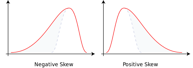
(From File:Negative and positive skew diagrams (English).svg - Wikipedia)
The fitting function is essentially a minimum discrepancy estimator. This means that the parameters of the parametric probability density function (PDF) are chosen to minimize the distance between the parametric PDF and the PDF formed by the data (the empirical PDF), for some specified metric of “distance”.
There are several measures of distance that could be used. For the purpose of this exploration of output age distribution forecasting, the distance metric to be minimized will be the total linear sum of the mass of the estimated parametric PDF that falls below the empirical PDF. With the “loss function” specified this way, the optimization algorithm attempts to minimize the probability that the real spends are much more likely to come from a block of a particular age compared to a potential decoy. Ideally, the decoy distribution would be identical to the real spend distribution, but parametric PDFs are not flexible enough to perfectly match an empirical PDF.
Define f_{S}(x) as the empirical spent output age distribution at block age x and f_{D}(x;\boldsymbol{\beta}) as a potential “decoy” distribution with some parameter vector \boldsymbol{\beta} (with the transparent blockchains presented here, there is no actual decoy mechanism of course). Then for each week of spent output age data the parameter vector \boldsymbol{\beta} can be chosen to minimize this quantity:
That is, minimize the sum of the difference between the real spend age distribution for blocks x_{i} where the decoy distribution is less than the real spend age distribution. The minimization is performed by computer numerical minimization methods similar to gradient descent.
The two candidate “decoy” parametric PDFs under consideration in this exercise are the Log-gamma (lgamma) distribution and the Right-Pareto Log-normal (rpln) distribution. The lgamma distribution, with two parameters, was used in Moser et al. (2018) to suggest a decoy distribution that was later incorporated into Monero’s reference wallet software. The rpln distribution is a more flexible distribution, with three parameters. The PDFs of these two distributions are:
with ratelog>0 and shapelog>0 and where \Gamma is the gamma function and
with shape2>0 and sdlog>0 and where \Phi is the cumulative distribution function of the standard Normal distribution.
Cross-blockchain correlations of summary statistics across time
The following table contains the correlation between several statistics over time for each pair of blockchains. The “BTC&BCH” correlation included data only for January 2018 onward to avoid artificially raising the correlation by including weeks when the BTC and BCH contained the same transaction before the August 2017 hard fork.
To be precise, define vector [x_{s,1},x_{s,2},\ldots,x_{s,W}]=\mathbf{X}_{s} for statistic s, e.g. the median, of blockchain x at each week, with W total weeks in the sample. Define \mathbf{Y}_{s} for blockchain y similarly. Then the quantities displayed in the table below are corr(\mathbf{X}_{s},\mathbf{Y}_{s}).
The two statistics that tend to have consistently high correlation for each pair of blockchains are skewness and kurtosis.
| statistic | BTC&BCH | BTC<C | BTC&DOGE | BCH<C | BCH&DOGE | LTC&DOGE |
|---|---|---|---|---|---|---|
| mean | -0.04 | -0.04 | -0.04 | -0.01 | -0.08 | 0.21 |
| median | -0.03 | -0.01 | -0.01 | -0.03 | -0.02 | -0.01 |
| sd | -0.07 | 0.02 | 0.34 | -0.02 | 0.02 | 0.35 |
| skewness | 0.09 | 0.24 | 0.19 | 0.11 | -0.32 | 0.28 |
| kurtosis | 0.02 | 0.29 | 0.31 | 0.22 | -0.26 | 0.23 |
| lgamma.shapelog | -0.05 | -0.23 | 0.12 | -0.05 | -0.01 | -0.02 |
| lgamma.ratelog | -0.02 | -0.14 | 0.13 | -0.03 | 0.00 | 0.02 |
| rpln.shape2 | 0.06 | -0.04 | -0.05 | 0.11 | -0.08 | 0.04 |
| rpln.meanlog | -0.03 | -0.14 | -0.04 | -0.19 | -0.11 | 0.15 |
| rpln.sdlog | 0.00 | 0.00 | 0.00 | -0.01 | 0.00 | -0.01 |

