
Irregular sampling for exponential moving average in DAA
Abstract
Averaging done in DAA is dependent on block production, that is irregular. Standard averaging techniques are designed to operate on data separated with regular time steps. This paper describes a method of averaging with irregular time sampling.
Introduction
Difficulty adjustment is a problem of measurement. An algorithm suitable for this task should adequately measure hashrate working on block production and apply the target that will result in the desired block production rate. A scheme using exponential moving average (EMA) is proposed^1 for this purpose. Because of stochastic nature of block production, the solve time, has to be averaged. Solve time is expressed in the units of \left[\frac{s}{\text{block}}\right] therefor the averaging sampling should occur once per block. Average time carries the information about the hashrate that was working on the chain over a smeared period of time, therefore, to adequately asses what hashing power was used to mine those blocks we should apply the same smoothing to the difficulties that were used for those blocks. Since now we are averaging hashrate that is in the units of \left[\frac{\text{hash}}{s}\right] our averaging should happen in regular time steps because of how exponential moving average is designed. Blocks come in irregular steps, especially during violent changes in the environment. We will answer the question how to modify the averaging procedure to take irregular time sampling into account.
Basic Exponential moving average
EMA formula lis as follows:
S_0=\frac{1p_0+(1-\alpha)p_1+(1-\alpha)^2p_2+(1-\alpha)^3 p_3\,+\,...}{1+(1-\alpha)+(1-\alpha)^2+(1-\alpha)^3\,+\,...}.\qquad\qquad(1)
The weights add up to unity (put p_i=1).
It can be expressed in a recursive form:
S_0=\frac{1p_0}{1+(1-\alpha)+(1-\alpha)^2+(1-\alpha)^3\,+\,...} + \frac{(1-\alpha)p_1+(1-\alpha)^2p_2+(1-\alpha)^3 p_3\,+\,...}{1+(1-\alpha)+(1-\alpha)^2+(1-\alpha)^3\,+\,...}=
=\frac{1p_0}{1+(1-\alpha)+(1-\alpha)^2+(1-\alpha)^3\,+\,...} + (1-\alpha)\frac{1p_1+(1-\alpha)p_2+(1-\alpha)^2 p_3\,+\,...}{1+(1-\alpha)+(1-\alpha)^2+(1-\alpha)^3\,+\,...}=
=\frac{1p_0}{1+(1-\alpha)+(1-\alpha)^2+(1-\alpha)^3\,+\,...}+(1-\alpha)S_0.
Additionally we have
\frac{1}{1+(1-\alpha)+(1-\alpha)^2+(1-\alpha)^3\,+\,...} = \left[\frac{1}{1-(1-\alpha)}\right]^{-1} = \alpha.
the final recursive formula is:
S_0= \alpha p_0 + (1-\alpha)S_1. \qquad\qquad(2)
Taking a next step in the moving average is equivalent to multiplying earlier terms by the factor (1-\alpha).
The above equation can be found as a constant time step discretization of a low-pass filter (read before continuing)
Regular sampling with different time step
Suppose we have to smoothing with a parameter \alpha_{\frac{1}{2}} that will be equivalent to smoothing with the parameter \alpha, but the sampling will be spaced by half the time as before.
we have the relation:
(1-\alpha_{\frac{1}{2}})=(1-\alpha)^{\frac{1}{2}}.\qquad\qquad (3)
The factor that multiplies the past measurements in the equation (1), when applied two times to the same data point, is squared and is equal to the weight that was used with slower sampling.
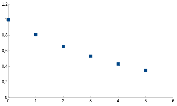
Figure 1. Weights when for (1-\alpha)=0.81.
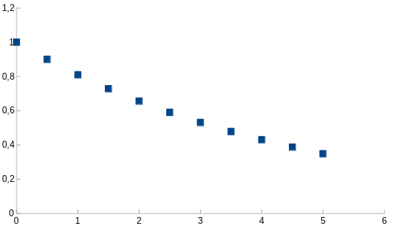
Figure 2. Weights for (1-\alpha_{\frac{1}{2}})=0.9, two times faster sampling.
We can see that weights from the Fig 1. are a subset of the weights in Fig 2.
Generalizing relation (3), we put the fraction of the initial time distance in the exponent.
(1-\alpha_{\frac{\Delta T_0}{\Delta T}})=(1-\alpha)^{\frac{\Delta T_0}{\Delta T}}.
Irregular sampling
Single irregular sample
Suppose we do a measurement once per second but we want want to change the distance between the most recent measurement and the measurement before it to be half of second. The expression for the average done this way will be:
S_0^{(1/2)}=\frac{1p_0+(1-\alpha)^{\frac{1}{2}}p_1+(1-\alpha)^{2+\frac{1}{2}}p_2+(1-\alpha)^{3+\frac{1}{2}} p_3\,+\,...}{1+(1-\alpha)^{\frac{1}{2}}+(1-\alpha)^{2+\frac{1}{2}}+(1-\alpha)^{3+\frac{1}{2}}\,+\,...} ,
and the weights are the following:
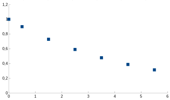
Figure 3. Weights with a single shorter time step.
Let us now transition to the recursive form.
S_0^{(1/2)}=\frac{1p_0+(1-\alpha)^{\frac{1}{2}}[p_1+(1-\alpha)^{2}p_2+(1-\alpha)^{3} p_3\,+\,...]}{1+(1-\alpha)^{\frac{1}{2}}[1+(1-\alpha)^{2}+(1-\alpha)^{3}\,+\,...]} =
= \frac{1p_0 +(1-\alpha)^{\frac{1}{2}}S_1/\alpha }{1+(1-\alpha)^{\frac{1}{2}}/\alpha} .
The first approximation we will use is (1+\varepsilon)^a\approx 1+a \varepsilon where \varepsilon is a small parameter.
S_0^{(1/2)}= \frac{1p_0 +(1-\alpha)^{\frac{1}{2}}S_1/\alpha }{1/\alpha+\frac{1}{2}}
Since \frac{1}{2} is small compared to 1/\alpha we do another approximation and end up with the recursive expression
S_0^{(1/2)}\approx\alpha p_0+(1-\alpha)^{\frac{1}{2}}S_1 .
The approximation error we made here is of the the order of \alpha^2.
As before, the formula can be generalized for any length of the time step.
S_0^{(\Delta T_0/\Delta T)}\approx\alpha p_0+(1-\alpha)^{\frac{\Delta T_0}{\Delta T}}S_1.
Ongoing Irregular sampling
The question that remains is can we do the irregular sampling over and over and keep the recurrent formula, modifying it to include the previous irregularly sampled average?
S_0^{(\Delta T_0/\Delta T)}\approx\alpha p_0+(1-\alpha)^{\frac{\Delta T_0}{\Delta T}}S_1^{(\Delta T_1/\Delta T)}. \qquad \qquad(4).
The answer is yes, as long as the average time is equal to \Delta T. N-th data point will be then weighted with (1-\alpha)^{N\frac{\Delta T_0+\Delta T_1+...+\Delta T_{N-1}}{N\Delta T}}. On each step a new error of the order \alpha^2 is committed, but this error is multiplied by (1-\frac{\Delta T_i}{\Delta T}) so as long as the steps are on average \Delta T, the errors cancel out. The higher order error does not cancel out and results in a small bias.
Unlike in the equation (2) the terms (1-\alpha)^{\frac{\Delta T_0}{\Delta T}} and \alpha do not add up to 1. This is necessary feature of this approach.
Difficulty adjustment context
In the context of difficulty adjustment, all the formulae have to use only integer mathematics. This requirement can be fulfilled by expanding the expression (1-\alpha)^{\frac{\Delta T_0}{\Delta T}} in Taylor series around the small parameter \alpha. It can be done to achieve arbitrary accuracy of the algorithm. The accuracy can be made larger than the nBits field in block header. (ref)
Experimental evaluation of irregular sampling DAA
The algorithm using nAvgSolveTime as described here was simulated in the Jonathan Toomim difficulty comparator both using regular sampling and irregular sampling (Fig. 4-8). The current DAA was also included in the experiment. Details of the experiment parameters will be listed in appendix.
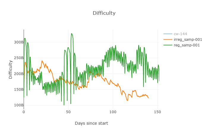
Figure 4. Difficulty of regular vs. irregular sampling in
nAvgSolveTime algorithm.
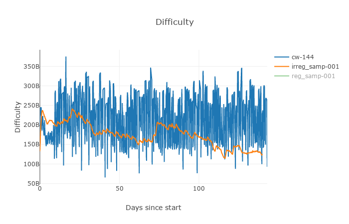
Figure 5. Difficulty of Irregular sampling in
nAvgSolveTime algorithm vs. the current BCH DAA.
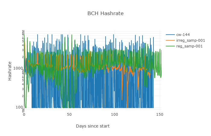
Figure 6. Hashrate changes resulting from the algorithms tested in the simulation.
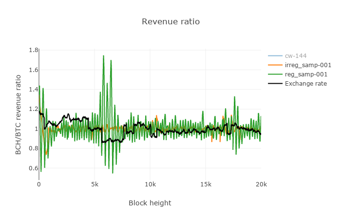
Figure 7. The ratio of incentives affecting switch mining.
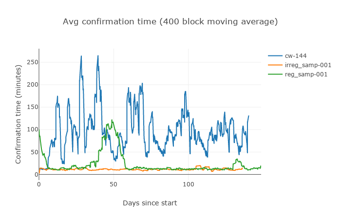
Figure 8.Average confirmation time from all three algorithms tested in the experiment.
Table 1. Mining strategy profitability.
| Algo | Profitability | ||
|---|---|---|---|
| greedy | variable | steady | |
| cw-144 | 9.74% | 5.719% | 3.839% |
| irreg_samp-001 | 0.60% | 0.110% | -0.306% |
| reg_samp-001 | 4.66% | 1.813% | 0.888% |
One may notice, that in the extreme conditions of this simulation the irregularly sampled algorithm performed very well, with little to no oscillations and kept the average block solve time around 10 min. The total time to solve 20000 blocks in simulation should have been 138 days and the regular algorithm made it almost perfectly, when both regular time and current DAA missed it a little.
Summary
The method to perform irregular sampling with exponential moving average has been derived (eq. 4) and tested. It is justified to use it as the method to adjust difficulty in blockchain, because blocks are produced in irregular time intervals.
Ackgnowledgements
I want to thank Jonathan Toomim firstly for creating the comparator, that is an amazing tools for modeling DAA, secondly for a hint how to use it, and lastly for making me realize that irregular time sampling might not be easily understandable at a first glance, even for a prepared observer, therefore there is a need to explain it better.
Appendix
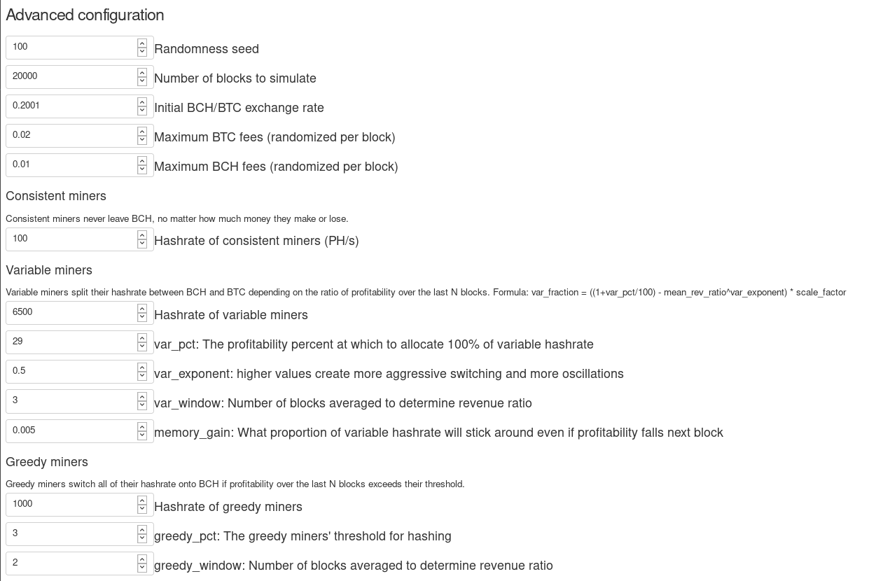
Figure 9. Simulation parameters.
